3 Peaks and Pits
“Peaks and Pits” is one of our fundamental project offerings and a workflow that is a solid representation of good data science work that we perform.
3.1 What is the concept/project background?
Strong memories associated to brands or products go deeper than simple positive or negative sentiment. Most of our experiences are not encoded in memory, rather what we remember about experiences are changes, significant moments, and endings. In their book “The Power of Moments”, two psychologists (Chip and Dan Heath) define these core memories as Peak and Pits, impactful experiences in our lives.
Broadly, peak moments are experiences that stand our memorable in our lives in a positive sense, whereas pit moments are impactful negative experiences.
Microsoft tasked us with finding a way to identify these moments in social data- going beyond ‘simple’ positive and negative sentiment which does not tell the full story of consumer/user experience. The end goal is that by providing Microsoft with these peak and pit moments in the customer experience, they can design peak moments in addition to simply removing pit moments.
The end goal
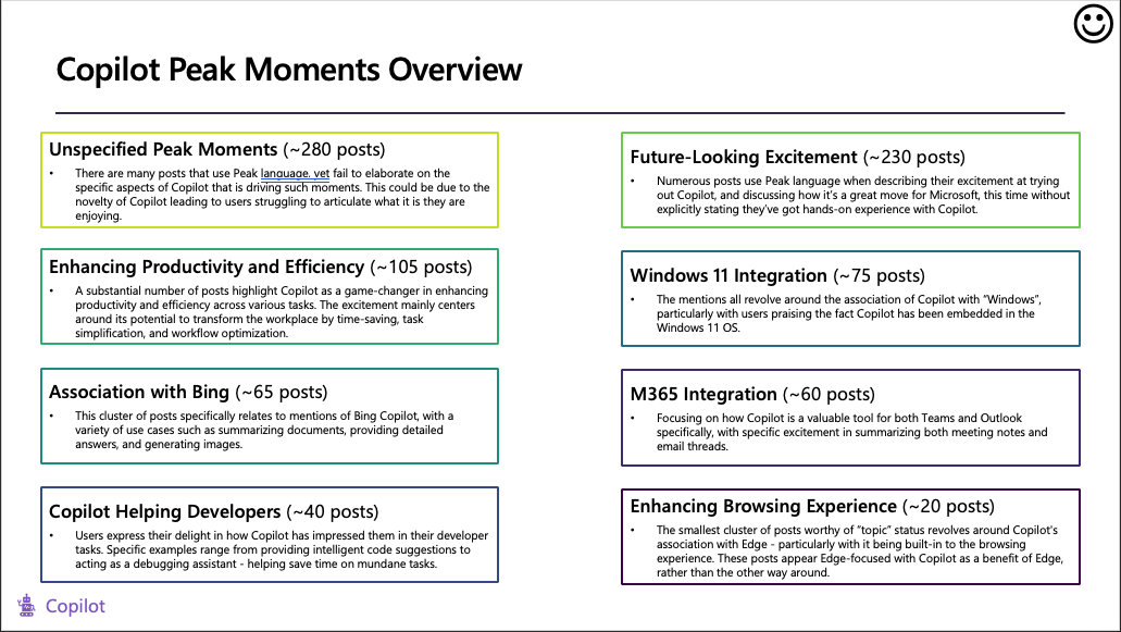
With these projects the core final ‘product’ is a collection of different peaks and pits, with suitable representative verbatims and an explanation to understand the high-level intricacies of these different emotional moments.
Key features of project
- There is no out-of-the-box ML model available whose purpose is to classify social media posts as either peaks or pits (i.e. we cannot use a ready-made solution, we must design our own bespoke solution).
- There is limited data available
- Unlike the case of spam/ham or sentiment classification, there is not a bank of pre-labelled data available for us to leverage for ‘traditional ML’.
- Despite these issues, the research problem itself is well defined (what are the core peak and pit moments for a brand/product), and because there are only three classes (peak, pit, or neither) which are based on extensive research, the classes themselves are well described (even if it is case of “you know a peak moment when you see it”).
3.2 Overview of approach
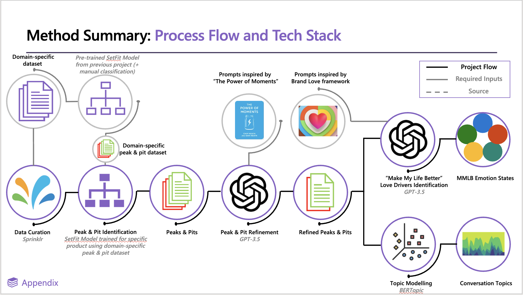
Peaks and pits projects have gone through many iterations throughout the past year and a half. Currently, the general workflow is to use utilise a model framework known as SetFit to efficiently train a text classification model with limited training data. This fine-tuned model is then able to run inference over large datasets to label posts as either peaks, pits, or neither. We then utilise the LLM capabilities to refine these peak and pit moments into a collection of posts we are extremely confident are peaks and/or pits. We then employ topic modelling to identify groups of similar peaks and pits to help us organise and discover hidden topics or themes within this collection of core moments.
This whole process can be split into six distinct steps:
- Extract brand/product mentions from Sprinklr (the start of any project)
- Obtain project-specific exemplar posts to help fine-tune a text classification model
- Perform model fine-tuning through contrastive learning
- Run inference over all of the project specific data
- Use GPT-3.5 for an extra layer of classification on identified peaks and pits
- Turn moments into something interpretable using topic modelling
Obtain posts for the project (Step 1)
This step relies on the analysts to export relevant mentions from Sprinklr (one of the social listening tools that analysts utilise to obtain social data), and therefore is not detailed much here. What is required is one dataset for each of the brands/products, so they can be analysed separately.
Identify project-specific exemplar peaks and pits to fine-tune our ML model (Step 2)
This step is synonymous with data labelling required for any machine learning project where annotated data is not already available.
Whilst there is no one-size-fits-all for determining the amount of data required to train a machine learning model, for traditional models and tasks, the number of examples per label is often in the region of thousands, and often this isn’t even enough for more complex problems.
The time required to accurately label thousands of peaks and pits to train a classification model in the traditional way is sadly beyond the scope of feasibility for our projects. As such we needed an approach that did not rely on copious amounts of pre-labelled data.
This is where SetFit comes in. As mentioned previously, SetFit is a framework that enables us to efficiently train a text classification model with limited training data.
Note the below is directly copied from the SetFit documentation. It is so succinctly written that trying to rewrite it would not do it justice.
Every SetFit model consists of two parts: a sentence transformer embedding model (the body) and a classifier (the head). These two parts are trained in two separate phases: the embedding finetuning phase and the classifier training phase. This conceptual guide will elaborate on the intuition between these phases, and why SetFit works so well.
Embedding finetuning phase
The first phase has one primary goal: finetune a sentence transformer embedding model to produce useful embeddings for our classification task. The Hugging Face Hub already has thousands of sentence transformer available, many of which have been trained to very accurately group the embeddings of texts with similar semantic meaning.
However, models that are good at Semantic Textual Similarity (STS) are not necessarily immediately good at our classification task. For example, according to an embedding model, the sentence of 1) “He biked to work.” will be much more similar to 2) “He drove his car to work.” than to 3) “Peter decided to take the bicycle to the beach party!”. But if our classification task involves classifying texts into transportation modes, then we want our embedding model to place sentences 1 and 3 closely together, and 2 further away.
To do so, we can finetune the chosen sentence transformer embedding model. The goal here is to nudge the model to use its pretrained knowledge in a different way that better aligns with our classification task, rather than making the completely forget what it has learned.
For finetuning, SetFit uses contrastive learning. This training approach involves creating positive and negative pairs of sentences. A sentence pair will be positive if both of the sentences are of the same class, and negative otherwise. For example, in the case of binary “positive”-“negative” sentiment analysis, (“The movie was awesome”, “I loved it”) is a positive pair, and (“The movie was awesome”, “It was quite disappointing”) is a negative pair.
During training, the embedding model receives these pairs, and will convert the sentences to embeddings. If the pair is positive, then it will pull on the model weights such that the text embeddings will be more similar, and vice versa for a negative pair. Through this approach, sentences with the same label will be embedded more similarly, and sentences with different labels less similarly.
Conveniently, this contrastive learning works with pairs rather than individual samples, and we can create plenty of unique pairs from just a few samples. For example, given 8 positive sentences and 8 negative sentences, we can create 28 positive pairs and 64 negative pairs for 92 unique training pairs. This grows exponentially to the number of sentences and classes, and that is why SetFit can train with just a few examples and still correctly finetune the sentence transformer embedding model. However, we should still be wary of overfitting.
Classifier training phase
Once the sentence transformer embedding model has been finetuned for our task at hand, we can start training the classifier. This phase has one primary goal: create a good mapping from the sentence transformer embeddings to the classes.
Unlike with the first phase, training the classifier is done from scratch and using the labelled samples directly, rather than using pairs. By default, the classifier is a simple logistic regression classifier from scikit-learn. First, all training sentences are fed through the now-finetuned sentence transformer embedding model, and then the sentence embeddings and labels are used to fit the logistic regression classifier. The result is a strong and efficient classifier.
Using these two parts, SetFit models are efficient, performant and easy to train, even on CPU-only devices.
There is no perfect number of labelled examples to find per class (i.e. peak, pit, or neither). Whilst in general more exemplars (and hence more training data) is beneficial, having fewer but high quality labelled posts is far superior than more posts of poorer quality. This is extremely important due to the contrastive nature of SetFit where it’s superpower is making the most of few, extremely good, labelled data.
Okay so now we know why we need labelled data, and we know what the model will do with it, what is our approach for obtaining the labelled data?
Broadly, we use our human judgement to read a post from the current project dataset, and manually label whether we think it is a peak, a pit, or neither. To avoid us just blindly reading through random posts in the dataset in the hope of finding good examples (this is not a good use of time), we can employ a couple of tricks to narrow our search region to posts that have a reasonable likelihood of being suitable examples.
The first trick is to use the OpenAI API to access a GPT model. This involves taking a sample of posts (say ~1000) and running these through a GPT model, with a prompt that asks the model to classify each post into either a peak, pit, or neither. This is possible because GPT models have learned knowledge of peaks and pits from its training on large datasets. We can therefore get a human to only sense-check/label posts that GPT also believes are peaks or pits.
The second trick involves using a previously created SetFit model (i.e. from an older project), and running inference over a similar sample of posts (again, say ~1000).
We would tend to suggest the OpenAI route, as it is simpler to implement (in our opinion), and often the old SetFit model has been finetuned on data from a different domain so it might struggle to understand domain specific language in the current dataset. However, be aware if it not as scalable as using an old SetFit model and has the drawback of being a prompt based classification of a black-box model (as well as issues relating to cost and API stability).
Irrespective of which approach is taken, by the end of this step we need to have a list of example posts we are confident represent what a peak or pit moment looks like for each particular product we are researching, including posts that are “neither”.
After so many projects now don’t we already have a good idea of what a peak and pit moment for the purposes of model training?
Each peak and pit project we work on has the potential to introduce ‘domain’ specific language, which a machine learning classifier (model) may not have seen before. By manually identifying exemplar peaks and pits that are project-specific, this gives our model the best chance to identify emotional moments appropriate to the project/data at hand.
The obvious case for this is with gaming specific language, where terms that don’t necessarily relate to an ‘obvious’ peak or pit moment could refer to one the gaming conversation, for example the terms/phrases “GG”, “camping”, “scrub”, and “goat” all have very specific meanings in this domain that differ from their use in everyday language.
Train our model using our labelled examples (Step 3)
Before we begin training our SetFit model with our data, it’s necessary to clean and wrangle the fine-tuning datasets. Specifically, we need to mask any mentions of brands or products to prevent bias. For instance, if a certain brand frequently appears in the training data within peak contexts, the model could erroneously link peak moments to that brand rather than learning the peak-language expressed in the text.
This precaution should extend to all aspects of our training data that might introduce biases. For example, as we now have examples from various projects, an overrepresentation of data from ‘gaming projects’ in our ‘peak’ posts within our training set (as opposed to the ‘pit’ posts) could skew the model into associating gaming-related language more with peaks than pits.
Broadly the cleaning steps that should be applied to our data for finetuning are:
- Mask brand/product mentions
- Remove hashtags #️⃣
- Remove mentions 💬
- Remove URLs 🌐
- Remove emojis 🐙
You will notice here we do not remove stop words-. As explained in the previous step, part of the finetuning process is to finetune a sentence embedding model, and we want to keep stop words so that we can use the full context of the post in order to finetune accurate embeddings.
At this step, we can split out our data into training, testing, and validation datasets. A good rule of thumb is to split the data 70% to training data, 15% to testing data, and 15% to validation data. By default, SetFit oversamples the minimum class within the training data, so we shouldn’t have to worry too much about imbalanced datasets- though be aware if we have extreme imbalanced we will end up sampling the same contrastive pairs (normally positive pairs) multiple times. However, our experimentation has shown that class imbalance doesn’t seem to have a significant effect to the training/output of the SetFit model for peaks and pits.
We are now at the stage where we can actually fine-tune the model. There are many different parameters we can change when fine-tuning the model, such as the specific embedding model used, the number of epochs to train for, the number of contrastive pairs of sentences to train on etc. For more details, please refer to the Peaks and Pits Playbook
We can assess model performance on the testing dataset by looking at accuracy, precision, recall, and F1 scores. For peaks and pits, the most important metric is actually recall because in step 4 we reclassify posts using GPT, so we want to make sure we are able to provide as many true peak/pit moments as possible to this step, even if it means we also provide a few false positives.
As a refresher, precision is the proportion of positive identifications that are actually correct (it focuses on the correctness of positive predictions) whereas recall is the proportion of actual positives that are identified correctly (it focuses on capturing all relevant instances).
In cases where false positives need to be minimised (incorrectly predicting a non-event as an event) we need to prioritise precision - if you’ve built a model to identify hot dogs from regular ol’ doggos, high precision ensures that normal dogs are not misclassified as hot dogs.
In cases where false negatives need to be minimised (failing to detect an actual event) we need to prioritise recall - in medical diagnoses we need to minimise the number of times a patient is incorrectly told they do not have a disease when in reality they do (or worded differently, we need to ensure that all patients with a disease are identified).
To apply this to our problem- we want to be sure that we capture all (or as many as possible) relevant instances of peaks or pits- even if a few false positives come in (neither posts that are incorrectly classified as peaks or pits). As we use GPT to make further peak/pit identifications, it’s better to provide GPT with with a comprehensive set of potential peaks and pits, including some incorrect ones, than to miss out on critical data.
Visualise model separation
As a bonus, we can actually neatly visualise how well our finetuning of the sentence transformer embedding model has gone- by seeing how well the model is able to separate our different classes in embedding space.
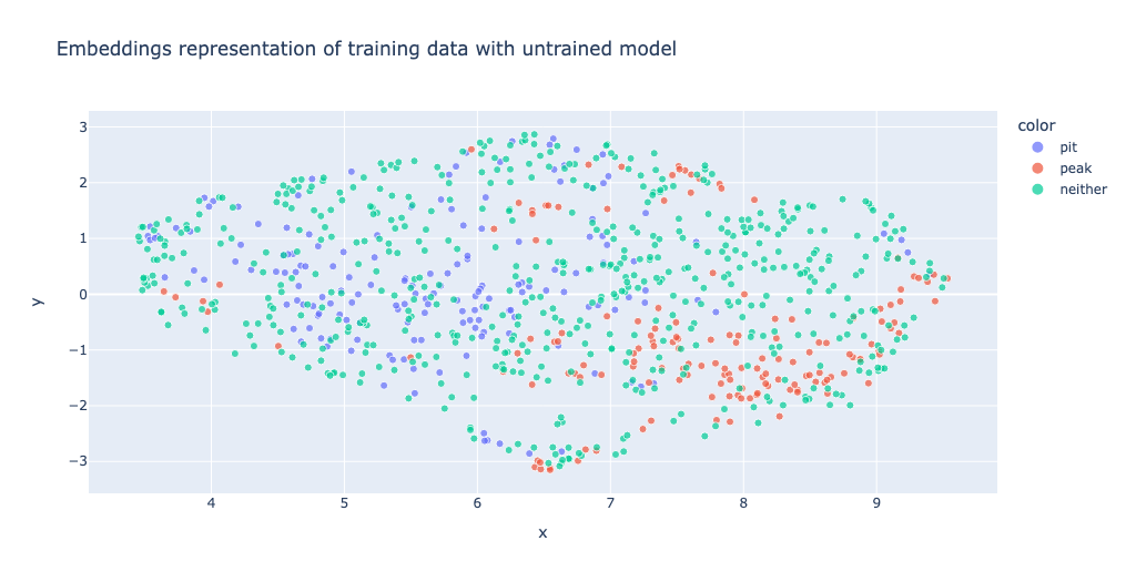
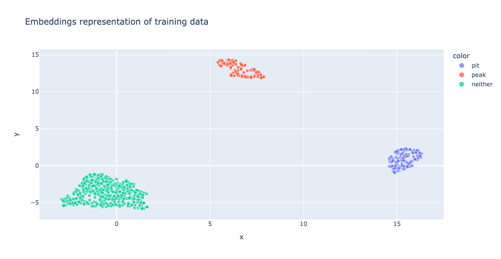
We can do this by visualising the 2-D structure of the embeddings and see how they cluster:
This is what it looks the embeddings space looks like on an un-finetuned model:
Here we can see that posts we know are peaks, pits, and neither all overlap and there is no real structure in the data. Any clustering of points observed are probably due to the posts’ semantic similarity (c.f. the mode of transport example above). We would not be able to nicely use a classifier model to get a good mapping from this embedding space to our classes (i.e. we couldn’t easily separate classes here).
By visualising the same posts after finetuning the embedding model, we get something more like this, where we can see that the embedding model now clearly separates posts based on their peak/pit classification (though we must be wary of overfitting!).
Finally, now we are happy with our model performance based on the training and validation datasets, we can evaluate the performance of this final model using our testing data. This is data that the model has never seen, and we are hoping that the accuracy and performance is similar to that of the validation data. This is Machine Learning 101 and if a refresher is needed for this there are plenty of resources online looking at the role of training, validation, and testing data.
Run inference over project data (Step 4)
It is finally time to infer whether the project data contain peaks or pits by using our fine-tuned SetFit model to classify the posts.
Before doing this again we need to make sure we do some data cleaning on the project specific data.
Broadly, this needs to match the high-level cleaning we did during fine-tuning stage:
- Mask brand/product mentions (using RoBERTa-based model [or similar] and
Rivendellfunctions) - Remove hashtags #️⃣
- Remove mentions 💬
- Remove URLs 🌐
- Remove emojis 🐙
Currently all peak and pit projects have been done on Twitter or Reddit data, but if a project includes web/forum data quirky special characters, numbered usernames, structured quotes etc. should also be removed.
Okay now we can finally run inference. This is extremely simple and only requires a couple of lines of code (again see the Peaks and Pits Playbook for code implementation)
The metal detector, GPT-3.5 (Step 5)
During step 4 we obtained peak and pit classification using few-shot classification with SetFit. The benefit of this approach (as outlined previously) is its speed and ability to classify with very few labelled samples due to contrastive learning.
However, during our iterations of peak and pit projects, we’ve realised that this step still classifies a fair amount of non-peak and pit posts incorrectly. This can cause noise in the downstream analyses and be very time consuming for us to further trudge through verbatims.
As such, the aim of this step is to further our confidence in our final list of peaks and pits to be actually peaks and pits. Remember before we explained that for SetFit, we focussed on recall being the most important measure in our business case? This is where we assume that GPT-3.5 enables us to remove the false positives due to it’s incredibly high performance.
Using GPT-3.5 for inference, even over relatively few posts as in peaks and pits, is expensive both in terms of time and money. Preliminary tests have suggested it is in the order of magnitude of thousands of times slower than SetFit. It is for these reasons why we do not use GPT-x models from the get go, despite it’s obvious incredible understanding of natural language.
Whilst prompt-based classification such as those with GPT-3.5 certainly has its drawbacks (dependency on prompt quality, prompt injections in posts, handling and version control of complex prompts, unexpected updates to the model weights rendering prompts ineffective), the benefits include increased flexibility in what we can ask the model to do. As such, in the absence of an accurate, cheap, and quick model to perform span detection, we have found that often posts identified as peaks/pits did indeed use peak/pit language, but the context of the moment was not related to the brand/product at the core of the research project.
For example, take the post that we identified in the project 706, looking for peaks and pits relating to PowerPoint:
This brings me so much happiness! Being a non-binary graduate student in STEM academia can be challenging at times. Despite using my they/them pronouns during introductions, emails, powerpoint presentations, name tags, etc. my identity is continuously mistaken. Community is key!
This is clearly a ‘peak’, however it is not accurate or valid to attribute this memorable moment to PowerPoint. Indeed, PowerPoint is merely mentioned in the post, but is not a core driver of the Peak which relates to feeling connection and being part of a community. This is as much a PowerPoint Peak as it is a Peak for the use of emails.
Therefore, we can engineer our prompt to include a caveat to say that the specific peak or pit moment must relate directly to the brand/product usage (if relevant).
Topic modelling to make sense of our data (Step 6)
Now we have an extremely refined set of posts classified as either peak or pits. The next step is to identify what these moments actually relate to (i.e. identify the topics of these moments through statistical methods).
To do this, we employ topic modelling via BERTopic to identifying high-level topics that emerge within the peak and pit conversation. This is done separately for each product and peak/pit dataset (i.e. there will be one BERTopic model for product A peaks, another BERTopic model for product A pits, an additional BERTopic model for product B peaks etc).
We implement BERTopic using the R package BertopicR. As there is already good documentation on BertopicR this section will not go into any technical detail in regards to implementation.
From BertopicR. we end up with a topic label for each post in our dataset, meaning we can easily quantify the size of each topics and visualise temporal patterns of topic volume etc.


